The following example will show you how to use SE::Pile to design a 24” octagonal prestressed concrete pile.

Pile dimension: 24” Octagonal

Clear cover: 2 inches

Concrete compressive strength: 8 ksi

Concrete ultimate strain: 0.003

Effective prestress: 1200psi

Strand: (22) 0.5” dia. 270ksi low relaxation seven wire strands

Confinement type: Spiral

Slenderness: unbraced length 60ft and effective length factor 1.0

Design load: P=300 kips, M = 200 k-ft

We use the Kip, in unit system by default.

Step 1

Draw an octagon which represents the outline of pile section with Draw–˃Shape–˃Regular Polygon.

Make the following changes for the octagon through property gird as shown in Figure 4.1.

Change CG of the octagon to (0, 0)

Change radius to 12”

Change number of sides to 8

Change Inscribed or circumscribed to inscribed

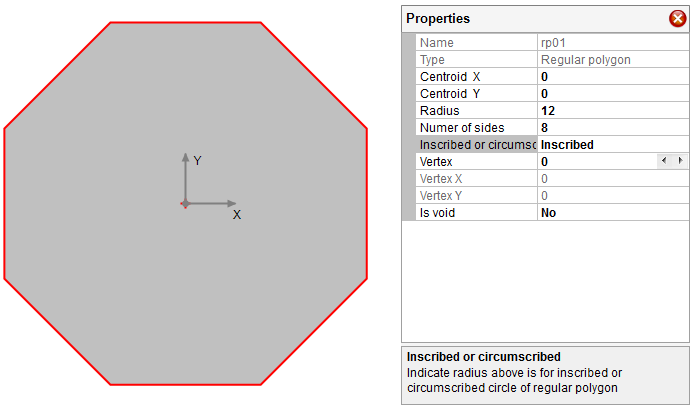
Figure 4.1 Step 1

Step 2

Draw pile strands with Draw–˃Reinforcement–˃Circular Pattern Bar. Make the following changes for the bar group through property gird as shown in Figure 4.2.

Change CG of the bar group to (0, 0)

Change circle diameter of the bar group to 19”

Change number of bars to 22

Change bar area to 0.153

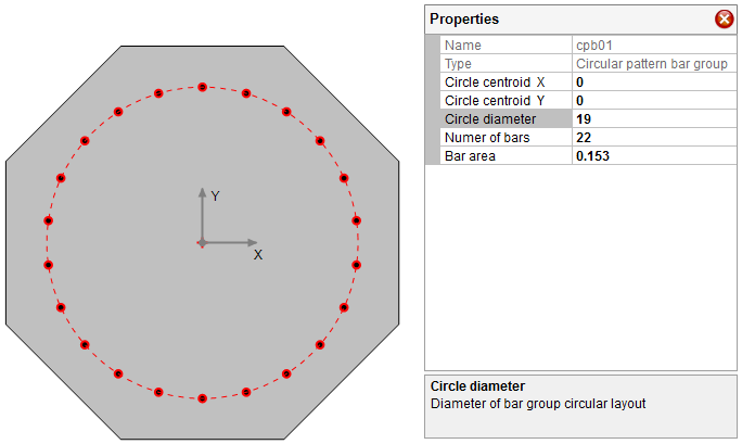
Figure 4.2 Step 2

Step 3

Input 8ksi for concrete strength and 0.003 for ultimate strain using Parameters–˃Concrete.

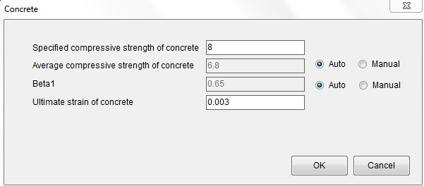
Figure 4.3 Step 3

Step 4

Input effective section prestress 1.2ksi and use the built in strand stress strain data using Parameters–˃Strand.

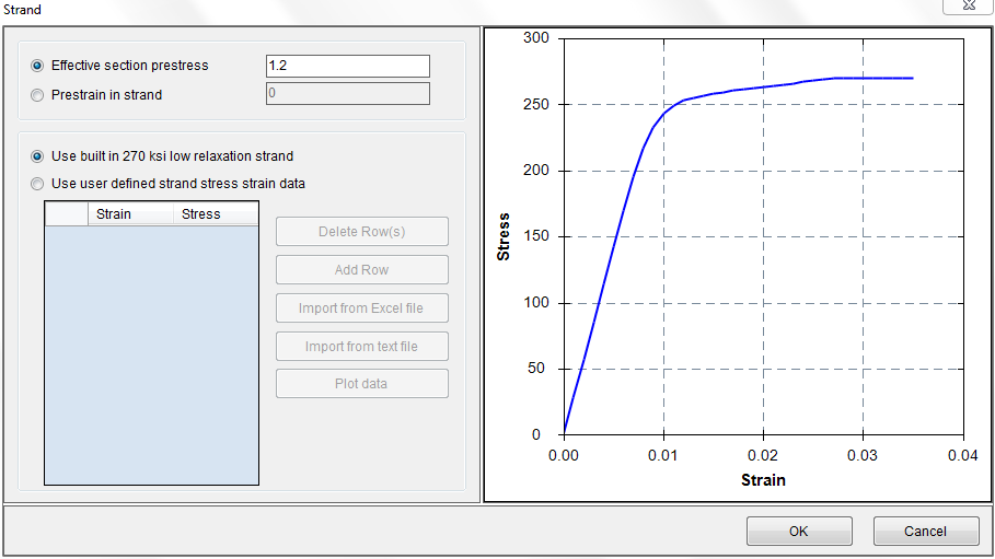
Figure 4.4 Step 4

Step 5

Input 1.0 for effective length factor and 720 in for unsupported length using Parameters–˃Slenderness

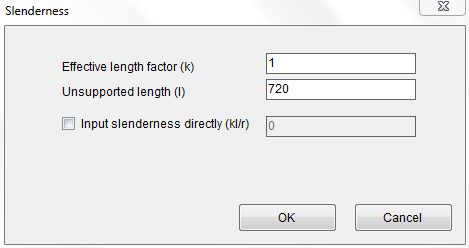
Figure 4.5 Step 5

Step 6

Select “Spiral” for the confinement type using Parameters–˃Resistance Factors

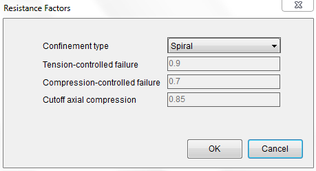
Figure 4.6 Step 6

Step 7

Switch unit system to Kip, ft. Input design loads using Parameters–˃Loads

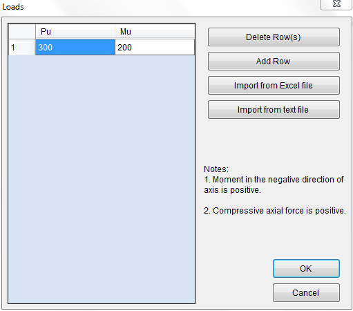
Figure 4.7 Step 7

Step 8

Now it is ready to run the analysis using Analysis–˃Run.

After analysis runs successfully, the output window will become active automatically as shown in Figure 4.8. The 1.147 C/D ratio means the pile is able to take the load.

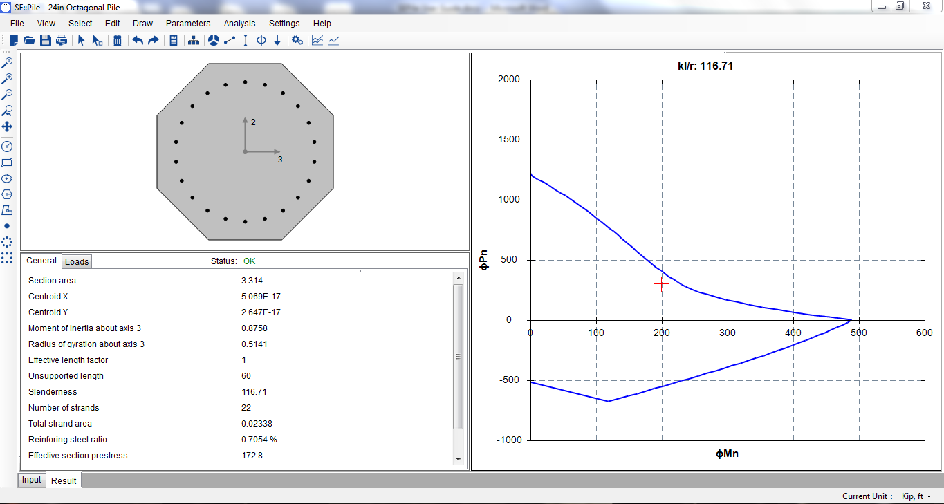
                    Figure 4.8 Output Window

Step 9

Finally, let’s plot the interaction diagrams for different slenderness. We want to plot from 0 to 200 with a step of 25.

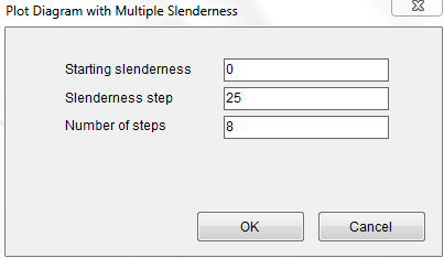
Figure 4.9.1 Step 9-1

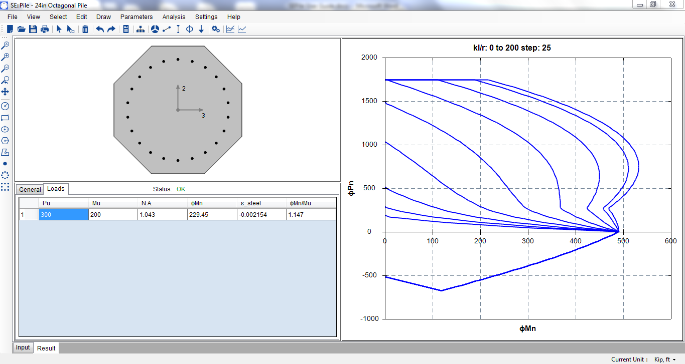
            Figure 4.9.2 Step 9-2