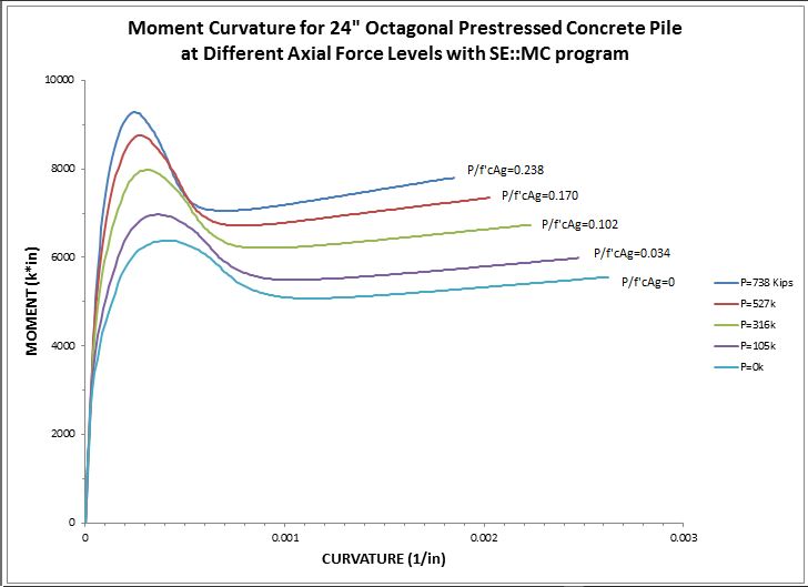
The following example will show you how to use SE::MC to perform moment curvature analysis for a 24” octagonal prestressed concrete pile section under different axial force levels. This example is from Chapter 12.5.3 of book Displacement-Based Seismic Design of Structures by M.J.N. Priestley et al. At the end, moment curvature curves for each axial force are plotted on a single chart to compare with curves published in the book.

Pile section: 24” octagonal

Clear cover: 3 inches

Confinement: W20 spiral @ 3” pitch   f_y=70ksi (yield strength) f_ye=70ksi(expected yield strength with over strength factor of 1.0)  ɛ_u=0.12(ultimate strain)

Concrete compressive strength: f’_c=6.5 ksi (compressive strength) f’_ce=1.3f’c=8.64ksi (expected compressive strength with over strength factor of 1.3)

Concrete tensile strength: 0 ksi

Concrete cover spalling strain: 0.005

Strands: (16) 0.6 in strands with A_s =0.215in²  f_pu=270ksi(ultimate strength)  f_pue=1.05f_pu=283.5ksi(expected ultimate strength with over strength factor of 1.05)

f_py=216ksi(yield strength)  ɛ_u=0.06(ultimate strain)

Initial strand stress after all losses: 154ksi

Modulus of elasticity: 29000ksi

Axial forces (Compression):

P/f’_cA_g=0.238  P=738kips

P/f’_cA_g=0.170  P=527kips

P/f’_cA_g=0.102  P=316kips

P/f’_cA_g=0.034  P=105kips

P/f’_cA_g=0         P=0kips

We use the Kip, in unit system by default.

Step 1

Draw an octagon which represents the outline of pile section with Draw–˃Shape–˃Regular Polygon.

Make sure the properties of the shape look the same as shown in Figure 1.0 except for material.

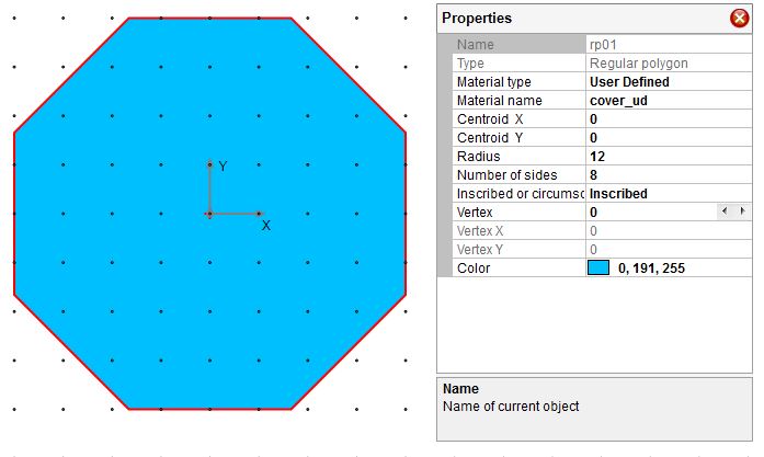
Figure 1.0 Step 1

Step 2

Draw a circle which represents the confined core of pile section with Draw–˃Shape–˃Circle. Make sure the properties of the shape look the same as shown in Figure 2.0 except for material.

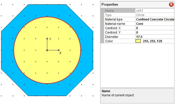
Figure 2.0 Step 2

Step 3

Draw strands with Draw–˃Reinforcement–˃Circular Pattern Bar. Make sure properties of the circular pattern bar look the same as shown in Figure 3.0 except for material. Prestrain is calculated by 154ksi/29000ksi= 0.00531. Prestrain is a negative value.

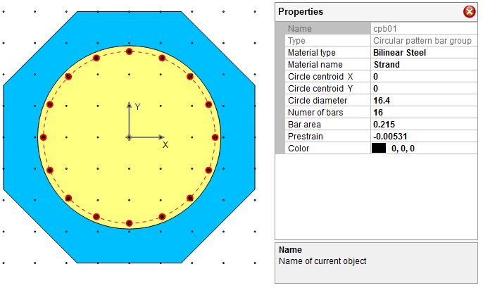
Figure 3.0 Step 3

Step 4

Define a material called “unconfined” with Material–˃Unconfined Concrete as shown in Figure 4.0. From the calculated stress strain data in the table, we can see that the maximum concrete compressive strain is 0.005. In order to allow the program to continue running after the concrete cover spalls off, we need to define the concrete stress strain data after strain reaches 0.005. We can do this by taking the calculated stress strain data here and create a user defined material called “cover_ud”. Let’s copy the stress strain data to an Excel file as shown in Figure 4.1. At the top, we need to add the headers “Strain” and “Stress”. We also need to add one more row of data “-1, 0” to define the tensile strain and stress. We typically don’t need to do this when we are using any built in material models since this is taken care of internally by the program. However, in the user defined material, the defined material fully relies on the user input. Finally, we need to add “0.1, 0” at the end of the last row. The reason we do this is to allow program to continuing running after concrete cover spalls off. The value “0.1” can be adjusted so that the final section failure is not controlled by the maximum cover compressive strain. However, this value cannot be too large because that will takes too long for the program to run. Define a user defined material called “cover” using Material–˃User Defined by importing the stress strain data in the Excel file as shown in Figure 4.2.

Figure 4.0 Step 4-1

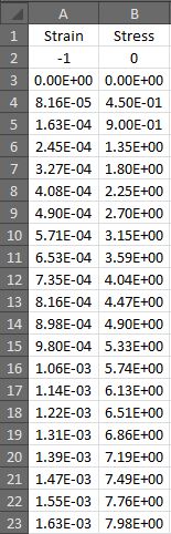
Figure 4.1 Step 4-2 (Not all data are shown)

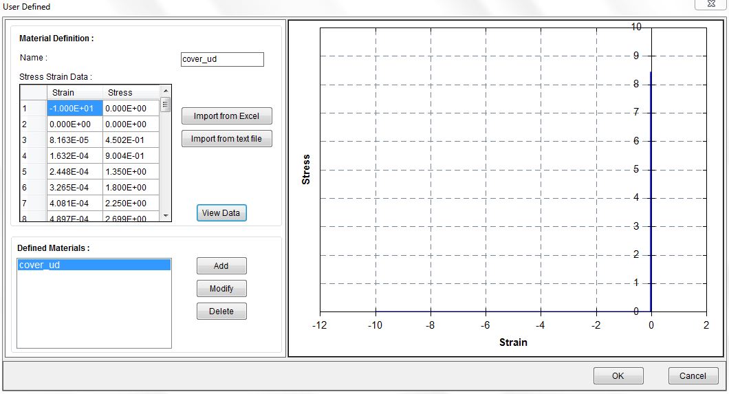
Figure 4.2 Step 4-3

Step 5

Define a material called “core” with Material–˃Confined Concrete Circular Section as shown in Figure 5.0.

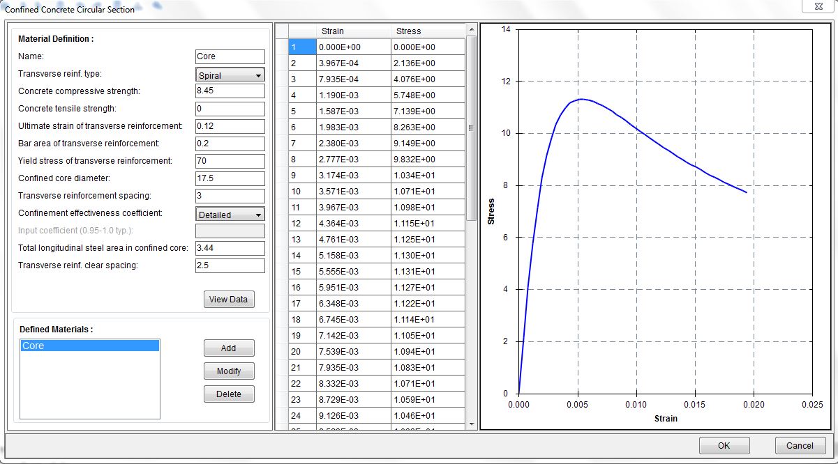
Figure 5.0 Confined Concrete Definition

Step 6

Here we use bilinear steel relationship to model the strand stress strain curve based on the information we have. Define a material called “Strand” with Material–˃Bilinear Steel as shown in Figure 6.0.

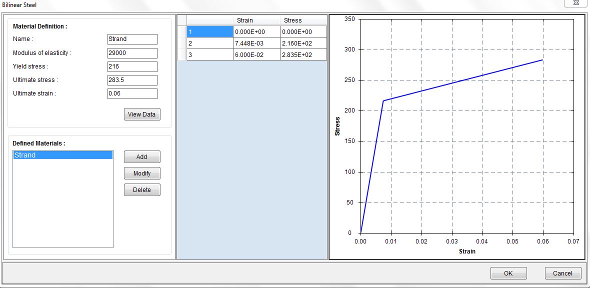
Figure 6.0 Strand

            Step 7

Assign the defined materials to the shapes and reinforcement through property grid. Here we only show the “cover_ud” material assignment for an example. After selecting the octagon in blue color, choose “User Defined” for material type and “cover_ud” for material name in the property grid. The other material assignments shall be done in a similar way.

Figure 7.0 Material Assignment

Step 8

Now it is ready to run the analysis using Analysis–˃Run. A dialog asking for axial force will pop up as show in Figure 4.8.1. Input 738 and click on the run button.

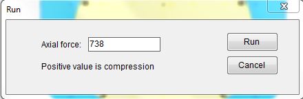
Figure 8.0 Axial Force Input Dialog

After analysis runs successfully, the output window will become active automatically as shown in Figure 8.1. You can view different results at each step of the analysis. Right click on the moment curvature chart and select export data to Excel to export the moment curvature data for this axial force.

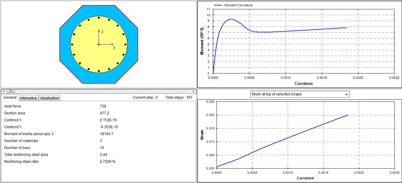
Figure 8.1 Output Window

Step 9

Repeat Step 8 for all other axial forces. After getting all the data, we can plot them in Excel as shown in Figure 9.0. The chart we have looks very similar to what the books shows. Due to copyright issues, we are not showing the chart from the book directly. You can always refer to the book for the chart.