The following example will show you how to use SE::MC to perform moment curvature analysis for a circular reinforced concrete column section. The concrete cover and confined core area will be modeled with unconfined concrete and confined concrete material models respectively.
Column diameter: 3 feet
Clear cover: 2 inches
Concrete compressive strength: 4 ksi (It is assumed that the over strength factor is 1.0 in this example)
Concrete tensile strength: 0 ksi
Concrete cover spalling strain: 0.005
Longitudinal reinforcement: 11#11 ASTM A706 fy = 60 ksi
Confinement: #5 spiral@4” spacing fy = 60ksi Ultimate strain = 0.12
Axial force: 1000kips compression
We use the Kip, in unit system by default.
Step 1
Draw a circle which represents the outline of column section with Draw–˃Shape–˃Circle.
Make the following changes for the circle through property gird as shown in Figure 4.1.
Change circle diameter to 36”
Change CG of the circle to (10, 10)
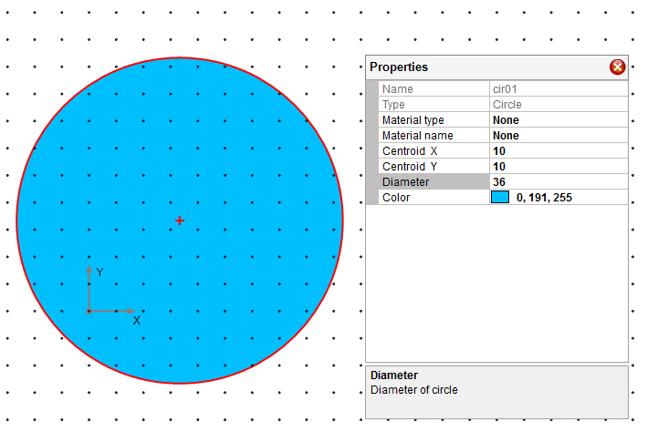
Figure 4.1 Step 1
Step 2
Draw another circle which represents the confined core of column section with Draw–˃Shape–˃Circle. Make the following changes for the circle through property gird as shown in Figure 4.2.
Change circle diameter to 32”
Change CG of the circle to (10, 10)
Change color of the circle to yellow
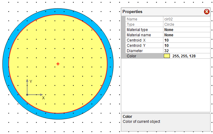
Figure 4.2 Step 2
Step 3
Draw column longitudinal reinforcement with Draw–˃Reinforcement–˃Circular Pattern Bar. Make the following changes for the bar group through property gird as shown in Figure 4.3.
Change diameter of the bar group to 30”
Change CG of the bar group to (10, 10)
Change number of bars to 11
Change bar area to 1.56
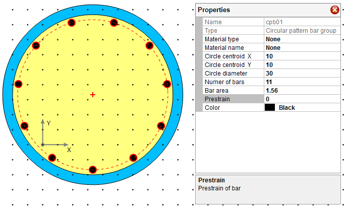
Figure 4.3 Step 3
Step 4
Define a material called “unconfined” with Material–˃Unconfined Concrete as shown in Figure 4.4.1. From the calculated stress strain data in the table, we can see that the maximum concrete compressive strain is 0.005. In order to allow the program to continue running after the concrete cover spalls off, we need to define the concrete stress strain data after strain reaches 0.005. We can do this by taking the calculated stress strain data here and create a user defined material called “cover”. Let’s copy the stress strain data to an Excel file as shown in Figure 4.4.2. At the top, we need to add the headers “Strain” and “Stress”. We also need to add one more row of data “-1, 0” to define the tensile strain and stress. We typically don’t need to do this when we are using any built in material models since this is taken care of internally by the program. However, in the user defined material, the defined material fully relies on the user input.
Finally, we need to add “0.1, 0” at the end of the last row. The reason we do this is to allow program to continuing running after concrete cover spalls off. The value “0.1” can be adjusted so that the final section failure is not controlled by the maximum cover compressive strain. However, this value cannot be too large because that will takes too long for the program to run.
Define a user defined material called “cover” using Material–˃User Defined by importing the stress strain data in the Excel file as shown in Figure 4.4-3.
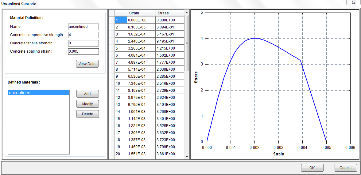
Figure 4.4.1 Step 4-1
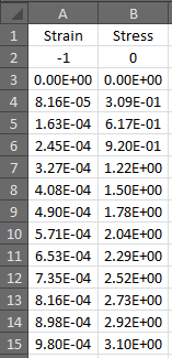
Figure 4.4.2 Step 4-2
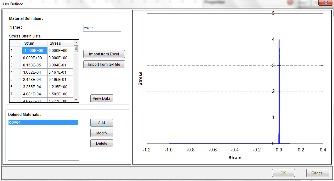
Figure 4.4.3 Step 4-3
Step 5
Define a material called “core” with Material–˃Confined Concrete Circular Section as shown in Figure 4.5.
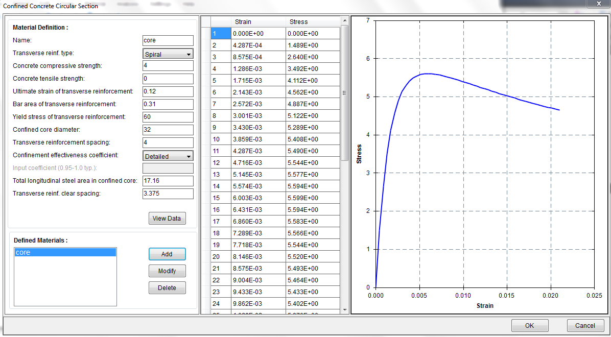
Figure 4.5 Confined Concrete Definition
Step 6
Define a material called “mild” with Material–˃Mild Steel as shown in Figure 4.6.
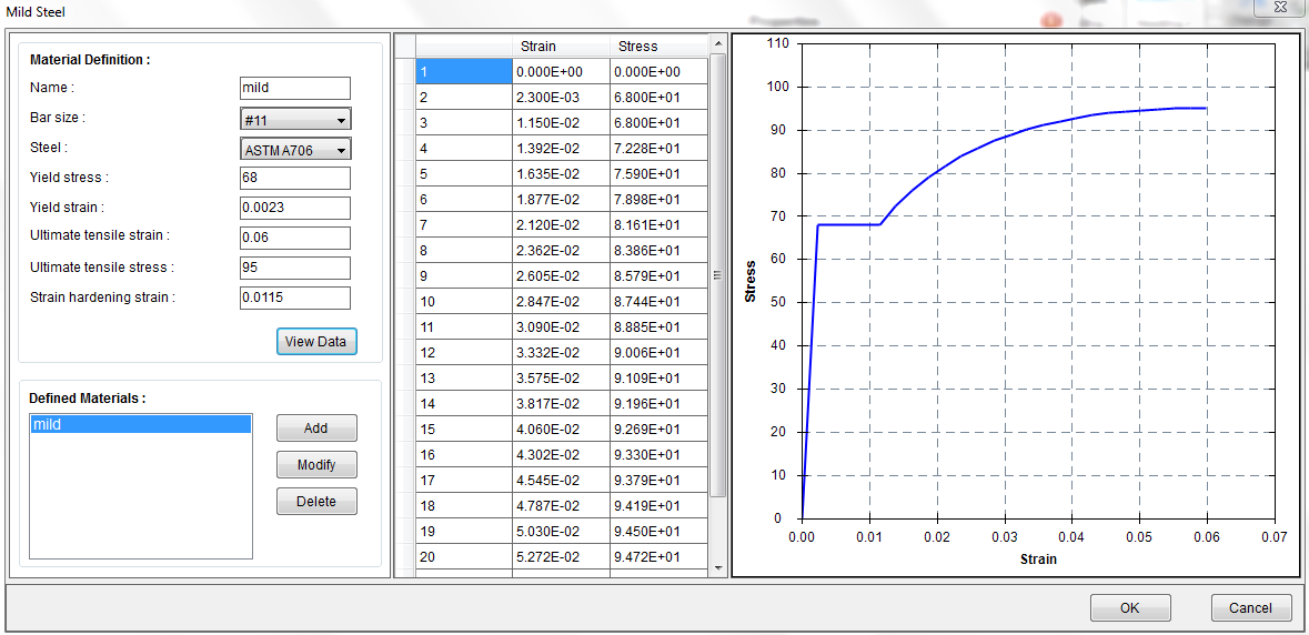
Figure 4.6 Mild Steel
Step 7
Assign the defined materials to the shapes and reinforcement through property grid. Here we only show the “cover” material assignment for an example. After selecting the larger circle in blue color, choose “User Defined” for material type and “cover” for material name in the property grid. The “core” and “mild” material assignment shall be done in a similar way.
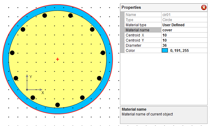
Figure 4.7 Material Assignment
Step 8
Now it is ready to run the analysis using Analysis–˃Run. A dialog asking for axial force will pop up as show in Figure 4.8.1. Input 1000 and click on the run button.
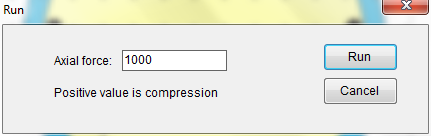
Figure 4.8.1 Axial Force Input Dialog
After analysis runs successfully, the output window will become active automatically as shown in Figure 4.8.2. You can view different results at each step of the analysis.
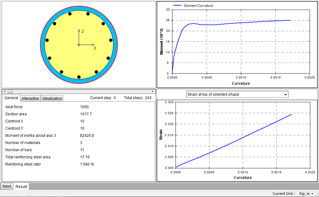
Figure 4.8.2 Output Window
Step 9
Finally, we will generate the idealized moment curvature analysis curve based on AASHTO Guide Specifications for LRFD Seismic Bridge Design using Analysis–˃Idealized Curve. We use the default values as shown in Figure 4.9.1. In many cases, you will need to input a smaller ultimate curvature which corresponds to the actual failure point determined by allowable strains from design criteria. Upon successful analysis, the idealized curve and data will be generated in the output window as shown in Figure 4.9.2. The data can be used to define plastic hinge for Pushover analysis in programs like SAP2000.
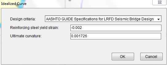
Figure 4.9.1 Generate Idealized Curve
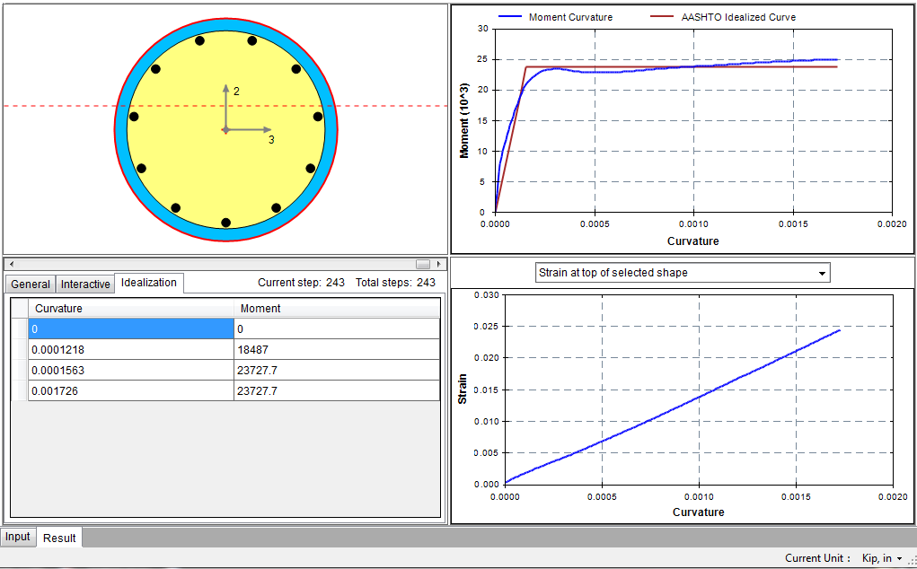
Figure 4.9.2 Idealized Curve